Systems of Linear Equations: Gaussian Elimination

It is quite hard to solve non-linear systems of equations, while linear systems are quite easy to study. There are numerical techniques which help to approximate nonlinear systems with linear ones in the hope that the solutions of the linear systems are close enough to the solutions of the nonlinear systems. We will not discuss this here. Instead, we will focus our attention on linear systems.

For the sake of simplicity, we will restrict ourselves to three, at most four, unknowns. The reader interested in the case of more unknowns may easily extend the following ideas.

Definition. The equation

a x + b y + c z + d w = h

where a, b, c, d, and h are known numbers, while x, y, z, and w are unknown numbers, is called a linear equation. If h =0, the linear equation is said to be homogeneous. A linear system is a set of linear equations and a homogeneous linear system is a set of homogeneous linear equations.

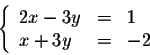
For example,

$$\left\{ \begin{array}{lll} 2x - 3y &=& 1\\ x+3y &=& -2\\ \end{array} \right.$$

and

$$\left\{ \begin{array}{lll} x+y-z &=& 1\\ x+3y + 3 z&=& -2\\ \end{array} \right.$$

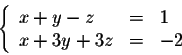
are linear systems, while

$$\left\{ \begin{array}{lll} 2x - 3y^2 &=& -1\\ x+y + z &=& 1\\ \end{array} \right.$$

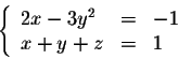
is a nonlinear system (because of y²). The system

$$\left\{ \begin{array}{lllllllll} 2x& - &3y& -&3 z &+ &w &=&0\\ x&+&3y&&&& &=& 0\\ x &-& y& +&&& w &=&0\\ \end{array} \right.$$

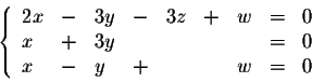
is an homogeneous linear system.

Matrix Representation of a Linear System

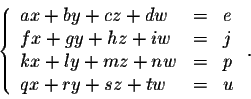
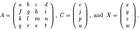
Matrices are helpful in rewriting a linear system in a very simple form. The algebraic properties of matrices may then be used to solve systems. First, consider the linear system

$$\left\{ \begin{array}{lllllll} ax + by + cz + dw &=& e\\ fx ... ... + nw &=& p\\ qx + ry + sz + tw &=& u\\ \end{array} \right. .$$

Set the matrices

$$A = \left( \begin{array}{lllllll} a& b& c& d\\ f& g& h&i\\ ... ...\begin{array}{lllllll} x\\ y\\ z\\ w\\ \end{array} \right).$$

Using matrix multiplications, we can rewrite the linear system above as the matrix equation

$$A\cdot X=C.$$

As you can see this is far nicer than the equations. But sometimes it is worth to solve the system directly without going through the matrix form. The matrix A is called the matrix coefficient of the linear system. The matrix C is called the nonhomogeneous term. When $C = {\cal O}$, the linear system is homogeneous. The matrix X is the unknown matrix. Its entries are the unknowns of the linear system. The augmented matrix associated with the system is the matrix [A|C], where

$$[A\vert C]= = \left( \begin{array}{llll \vert l} a& b& c& d&e... ...& g& h&i&f\\ k& l& m&n&p\\ q&r&s& t&u\\ \end{array} \right).$$

In general if the linear system has n equations with m unknowns, then the matrix coefficient will be a nxm matrix and the augmented matrix an nx(m+1) matrix. Now we turn our attention to the solutions of a system.

Definition. Two linear systems with n unknowns are said to be equivalent if and only if they have the same set of solutions.

This definition is important since the idea behind solving a system is to find an equivalent system which is easy to solve. You may wonder how we will come up with such system? Easy, we do that through elementary operations. Indeed, it is clear that if we interchange two equations, the new system is still equivalent to the old one. If we multiply an equation with a nonzero number, we obtain a new system still equivalent to old one. And finally replacing one equation with the sum of two equations, we again obtain an equivalent system. These operations are called elementary operations on systems. Let us see how it works in a particular case.

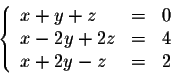
Example. Consider the linear system

$$\left\{ \begin{array}{lll} x+y+z&=& 0\\ x-2y + 2z&=& 4\\ x+2y -z&=& 2\\ \end{array} \right.$$

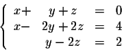
The idea is to keep the first equation and work on the last two. In doing that, we will try to kill one of the unknowns and solve for the other two. For example, if we keep the first and second equation, and subtract the first one from the last one, we get the equivalent system

$$\left\{ \begin{array}{ccccccc} x+&y+z&=& 0\\ x-&2y + 2z&=& 4\\ &y -2z&=& 2\\ \end{array} \right.$$

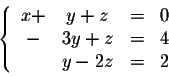
Next we keep the first and the last equation, and we subtract the first from the second. We get the equivalent system

$$\left\{ \begin{array}{ccccccc} x+&y+z&=& 0\\ -&3y + z&=& 4\\ &y -2z&=& 2\\ \end{array} \right.$$

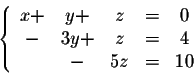
Now we focus on the second and the third equation. We repeat the same procedure. Try to kill one of the two unknowns (y or z). Indeed, we keep the first and second equation, and we add the second to the third after multiplying it by 3. We get

$$\left\{ \begin{array}{ccccccc} x+&y+&z&=& 0\\ -&3y + &z&=& 4\\ &-&5z&=& 10\\ \end{array} \right.$$

This obviously implies z = -2. From the second equation, we get y = -2, and finally from the first equation we get x = 4. Therefore the linear system has one solution

$$x=4,\; y = -2,\; z = -2.$$

Going from the last equation to the first while solving for the unknowns is called backsolving.

Keep in mind that linear systems for which the matrix coefficient is upper-triangular are easy to solve. This is particularly true, if the matrix is in echelon form. So the trick is to perform elementary operations to transform the initial linear system into another one for which the coefficient matrix is in echelon form.
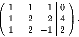
Using our knowledge about matrices, is there anyway we can rewrite what we did above in matrix form which will make our notation (or representation) easier? Indeed, consider the augmented matrix

$$\left( \begin{array}{rrr\vert r} 1&1&1& 0\\ 1&-2&2& 4\\ 1&2&-1& 2\\ \end{array} \right).$$

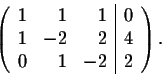
Let us perform some elementary row operations on this matrix. Indeed, if we keep the first and second row, and subtract the first one from the last one we get

$$\left( \begin{array}{rrr\vert r} 1&1&1& 0\\ 1&-2&2& 4\\ 0&1&-2& 2\\ \end{array} \right).$$

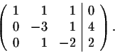
Next we keep the first and the last rows, and we subtract the first from the second. We get

$$\left( \begin{array}{rrr\vert r} 1&1&1& 0\\ 0&-3&1& 4\\ 0&1&-2& 2\\ \end{array} \right).$$

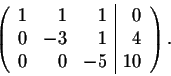
Then we keep the first and second row, and we add the second to the third after multiplying it by 3 to get

$$\left( \begin{array}{rrr\vert r} 1&1&1& 0\\ 0&-3&1& 4\\ 0&0&-5& 10\\ \end{array} \right).$$

This is a triangular matrix which is not in echelon form. The linear system for which this matrix is an augmented one is

$$\left\{ \begin{array}{ccccccc} x+&y+&z&=& 0\\ -&3y + &z&=& 4\\ &-&5z&=& 10\\ \end{array} \right.$$

As you can see we obtained the same system as before. In fact, we followed the same elementary operations performed above. In every step the new matrix was exactly the augmented matrix associated to the new system. This shows that instead of writing the systems over and over again, it is easy to play around with the elementary row operations and once we obtain a triangular matrix, write the associated linear system and then solve it. This is known as Gaussian Elimination. Let us summarize the procedure:

Gaussian Elimination. Consider a linear system.

1.

Construct the augmented matrix for the system;

2.

Use elementary row operations to transform the augmented matrix into a triangular one;

3.

Write down the new linear system for which the triangular matrix is the associated augmented matrix;

4.

Solve the new system. You may need to assign some parametric values to some unknowns, and then apply the method of back substitution to solve the new system.

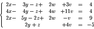
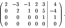
Example. Solve the following system via Gaussian elimination

$$\left\{ \begin{array}{ccccccc} 2x-&3 y-z + &2w& + 3 v&=&4\\ ... ...+ &2w& - v &=&9\\ &2y + z &&+ 4 v &=&-5\\ \end{array} \right.$$

The augmented matrix is

$$\left( \begin{array}{rrrrr\vert r} 2&-3&-1& 2&3&4\\ 4&-4&-1&... ...1&4\\ 2&-5&-2& 2&-1&9\\ 0&2&1& 0&4&-5\\ \end{array} \right).$$

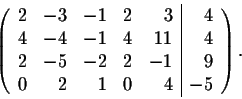
We use elementary row operations to transform this matrix into a triangular one. We keep the first row and use it to produce all zeros elsewhere in the first column. We have

$$\left( \begin{array}{rrrrr\vert r} 2&-3&-1& 2&3&4\\ 0&2&1& 0&5&-4\\ 0&-2&-1& 0&-4&5\\ 0&2&1& 0&4&-5\\ \end{array} \right).$$

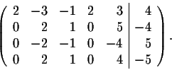
Next we keep the first and second row and try to have zeros in the second column. We get

$$\left( \begin{array}{rrrrr\vert r} 2&-3&-1& 2&3&4\\ 0&2&1& 0&5&-4\\ 0&0&0& 0&1&1\\ 0&0&0& 0&-1&-1\\ \end{array} \right).$$

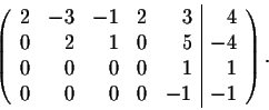
Next we keep the first three rows. We add the last one to the third to get

$$\left( \begin{array}{rrrrr\vert r} 2&-3&-1& 2&3&4\\ 0&2&1& 0&5&-4\\ 0&0&0& 0&1&1\\ 0&0&0& 0&0&0\\ \end{array} \right).$$

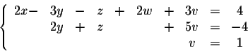
This is a triangular matrix. Its associated system is

$$\left\{ \begin{array}{cccccccccc} 2x-&3 y&-&z &+ &2w& + &3 v&=&4\\ &2y&+&z &&&+&5 v&=&-4\\ &&&&&&&v&=&1 \end{array} \right.$$

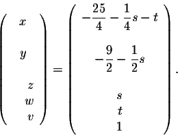
Clearly we have v = 1. Set z=s and w=t, then we have

$$y = -2 -\frac{1}{2} z - \frac{5}{2} v = -\frac{9}{2} - \frac{1}{2} s.$$

The first equation implies

x = 2 + $${\frac{{3}}{{2}}}$$y + $${\frac{{1}}{{2}}}$$z - w - $${\frac{{3}}{{2}}}$$v.

Using algebraic manipulations, we get

x = - $${\frac{{25}}{{4}}}$$ - $${\frac{{1}}{{4}}}$$s - t.

Putting all the stuff together, we have

$$\left( \begin{array}{rrrrrrr} \phantom{\frac{1}{1}}x\phantom{... ...{2} - \frac{1}{2} s\\ \\ s\\ t\\ 1\\ \end{array} \right) .$$

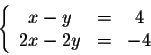
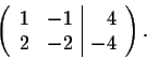
Example. Use Gaussian elimination to solve the linear system

$$\left\{ \begin{array}{cccccc} x - y &=&4\\ 2x - 2y&=&-4\\ \end{array} \right.$$

The associated augmented matrix is

$$\left( \begin{array}{rr\vert r} 1&-1&4\\ 2&-2&-4\\ \end{array} \right).$$

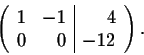
We keep the first row and subtract the first row multiplied by 2 from the second row. We get

$$\left( \begin{array}{rr\vert r} 1&-1&4\\ 0&0&-12\\ \end{array} \right).$$

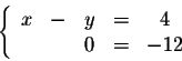
This is a triangular matrix. The associated system is

$$\left\{ \begin{array}{cccccc} x &- &y &=&4\\ &&0&=&-12\\ \end{array} \right.$$

Clearly the second equation implies that this system has no solution. Therefore this linear system has no solution.

Definition. A linear system is called inconsistent or overdetermined if it does not have a solution. In other words, the set of solutions is empty. Otherwise the linear system is called consistent.

Following the example above, we see that if we perform elementary row operations on the augmented matrix of the system and get a matrix with one of its rows equal to 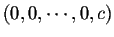$(0,0,\cdots,0,c)$, where $c \neq 0$, then the system is inconsistent.

[Back] [Next] [Geometry] [Algebra] [Trigonometry ] [Calculus] [Differential Equations] [Matrix Algebra]

S.O.S MATH: Home Page

Do you need more help? Please post your question on our S.O.S. Mathematics CyberBoard.

Author: M.A. Khamsi

Copyright © 1999-2024 MathMedics, LLC. All rights reserved.
Contact us
Math Medics, LLC. - P.O. Box 12395 - El Paso TX 79913 - USA
users online during the last hour