 Introduction and Motivation
 Introduction and Motivation

The differential equations are very much helpful in many areas of
science. But most of interesting real life problems involve more than
one unknown function. Therefore, the use of system of differential
equations is very useful. Without loss of generality, we will
concentrate on systems of two differential equations

As a motivation let us consider an island with two type of species: Rabbits and Fox. Clearly one plays the role of predator while the other one the role of a prey. If we are interested to model the populations growths of both species, then we have to keep in mind that if, for example, the population of the Fox increases, then the Rabbit population will be affected. So the rate of change of the population of one type will depend on the actual population of the other type. For example, in the absence of the Rabbit population, the Fox population will decrease (and fast) to face a certain extinction. Something that most of us would like to avoid. A model for this Predator-Prey problem was developed by Lotka (in 1925) and Volterra (in 1926) and is known as the Lotka-Volterra system

where R(t) measures the Rabbit population, F(t) measures the Fox
population, and all the involved constant ![]() are
positive numbers. Note that a and b are the growth rate of the
prey, and the death rate of the predator.
are
positive numbers. Note that a and b are the growth rate of the
prey, and the death rate of the predator. ![]() and
and ![]() are
measures of the effect of the interaction between the Rabbits and The
Fox.
are
measures of the effect of the interaction between the Rabbits and The
Fox.
Note that in the Lotka-Volterra system, the variable t is missing. This kind of system is called autonomous system and are written

Phase Plane
Let us go back to the general case

A solution to this system is the couple of functions (x(t),y(t)) which satisfy both differential equations of the system. When we change the variable t, then we get a set of points on the xy-plane which, in physics, we usually call a trajectory. The moving object has the coordinates (x(t),y(t)) at time t. The velocity to the trajectory at time t is given by
![]()
Note that we do not need to know the solution (x(t),y(t) to determine the velocity vector at time t. Indeed, we have
![]()
as long as we know x, y, and t. In particular, we can draw all
the velocity vectors everywhere on the plane for the autonomous
systems. This is known as the vector field.
The vector field should be understood as the analogue of
the direction field for differential equations.
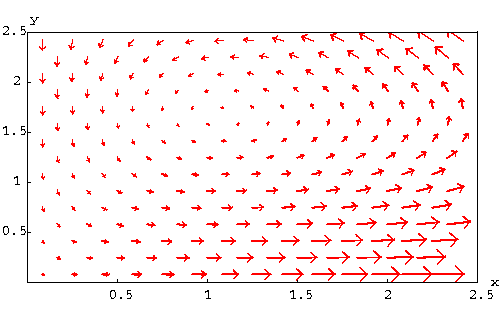
Example. Draw the vector field for the predator-prey problem

For example, for the point (x,y)= (2,1), we have
![]()
If we put more velocity vectors, we get
|
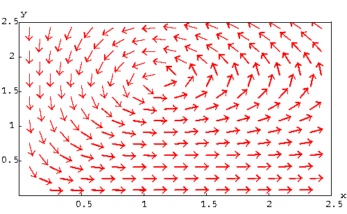
It is clear that the length of the velocity vectors may affect our
understanding of the solutions. If we are only interested by the
direction of the motion not its speed, then it is natural to fix a
length for these vectors
|
Compare the two pictures.
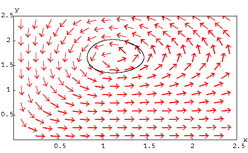
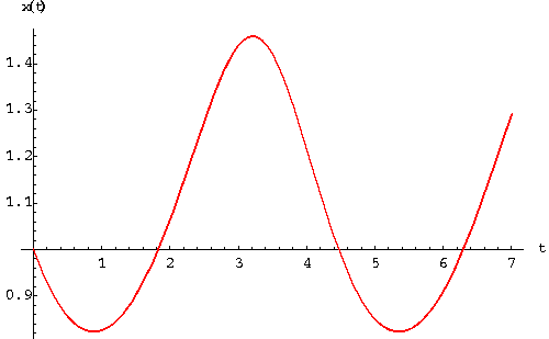
Remark. Note that for the predator-prey problem, we may be interested to find out whether one of the two species is facing extinction or not. In other words, we may be interested to study the functions x(t) and y(t) separately. In other words, two more graphs are naturally associated to a system. For the above example, the graph of the solution which satisfies the condition
![]()
is drawn below
|
and the graphs of x(t) and y(t) are
|
and
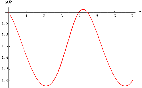
|
Equilibrium Solutions.
An equilibrium solution (or critical solution) of an
autonomous system is the trajectory of a moving-object with no motion,
that is the object is not moving. In this case, the velocity vector
is basically equal to 0. Consider the autonomous system

The equilibrium solutions are the algebraic solutions of the system
![]()
The equilibrium solutions are also called equilibrium points since the associated trajectories are exactly points on the phase plane.
Example. Find the equilibrium points of the Duffin system

Answer. We consider the system
![]()
Plugging y=0 in the second equation, we get
![]()
which gives x = 0, or ![]() . Hence the equilibrium points are
. Hence the equilibrium points are
![]()

 S.O.S MATHematics home page
 Do you need more help? Please post your question on our S.O.S. Mathematics CyberBoard.

Author: Mohamed Amine Khamsi